A* Path Planing

• Skills: A star algorithm, Python, Path planing, Navigation
• Course project

---

Demo:

Figure 1: A_star search path planing and robot navigation

Overall:

This project develop an online and offline implementation of A* search algorithm to generate a 2-D path which navigates while avoiding obstacles, and design a inverse kinematics controller to drive a differential wheeled robot to drive along the path.

Details:

A* is an informed search algorithm, or a best-first search, meaning that it is formulated in terms of weighted graphs: starting from a specific starting node of a graph, it aims to find a path to the given goal node having the smallest cost. It does this by maintaining a tree of paths originating at the start node and extending those paths one edge at a time until its termination criterion is satisfied. At each iteration of its main loop, A* needs to determine which of its paths to extend. It does so based on the cost of the path and an estimate of the cost required to extend the path all the way to the goal. Specifically, A* selects the path that minimizes :

\begin{equation}\label{final_transform} f(n) = g(n) +h(n) \end{equation} \(g(n)\) is true cost. We define true cost = +1 move into a neighbor cell that is unoccupied, and true cost = 1000 to move into a neighbor cell that is occupied. There are 15 landmarks,which means there are 15 occupied cells.

\(h(n)\) is heuristic, applying Euclidean distance estimated distance from the current node to the end node. The obstacle true cost is much greater than heuristic value. With this heuristic, we can make sure that we can actually calculate it and its admissible. It’s also very important that this heuristic is always an underestimation of the total path, as an overestimation will lead to A* searching for through nodes that may not be the ‘best’ in terms of f value.

\(f(n)\) is the total cost. A* is the algorithm prioritizes the node with the lowest f and the ‘best’ chance of reaching the end.

Offline:

Robot start from the original point, and use original point as the current point, this current point would have children as 8 neighbors, and add all children to the open list. Then robot need to pick a node with smallest \(f(n)\) from the open list, if more than one node have same smallest value of \(f(n)\), then robot would pick a node which has smaller \(g(n)\) and add this node to the close list, and delete this node from the open list. Also robot would use this node to update current node, and use the same method to keep update the current node until it match with the goal. The last step to trace back its parents to find the path.

Figure 3: Plan path base on A star algorithm (a):S =[0.5,-1.5],G = [0.5,1.5], (b): s=[4.5,3.5], G =[4.5,- 1.5], (c):S = [-0.5, 5.5],G = [1.5, -3.5]

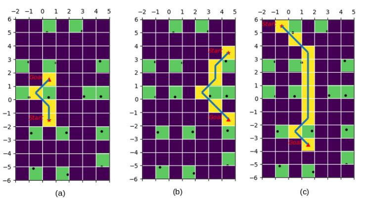
The figure 3 shows the A star offline path planing, which begin from the start point to the end point, the green boxes are the obstacles, the yellow blocks are the path planned while avoiding obstacles.

Online:

Online A* code: when robot at the start point, robot using question 2 code to find the best cost node which has smallest f(n) among its neighbors. Then robot use this best node to replace its start point, which means robot then would start from this best node, then go through question online code again to find next best cost among its neighbor and update new start point. robot would keep doing this method until its new start point match its goal. All start points would be the path of Online A* code. So unlike the offline code, the open list for the online A* would only contain the 8 neighbors of current start point.

Figure 4: Plan path base on A star algorithm (a):S =[0.5,-1.5],G = [0.5,1.5], (b): s=[4.5,3.5], G =[4.5,- 1.5], (c):S = [-0.5, 5.5],G = [1.5, -3.5]

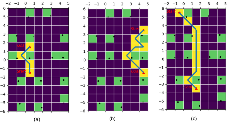
The figure 4 shows the A star offline path planing, which begin from the start point to the end point, the grid size is \(1m \times 1 m\) the green boxes are the obstacles, the yellow blocks are the path planned while avoiding obstacles.

Realistic grid and Robot navigation

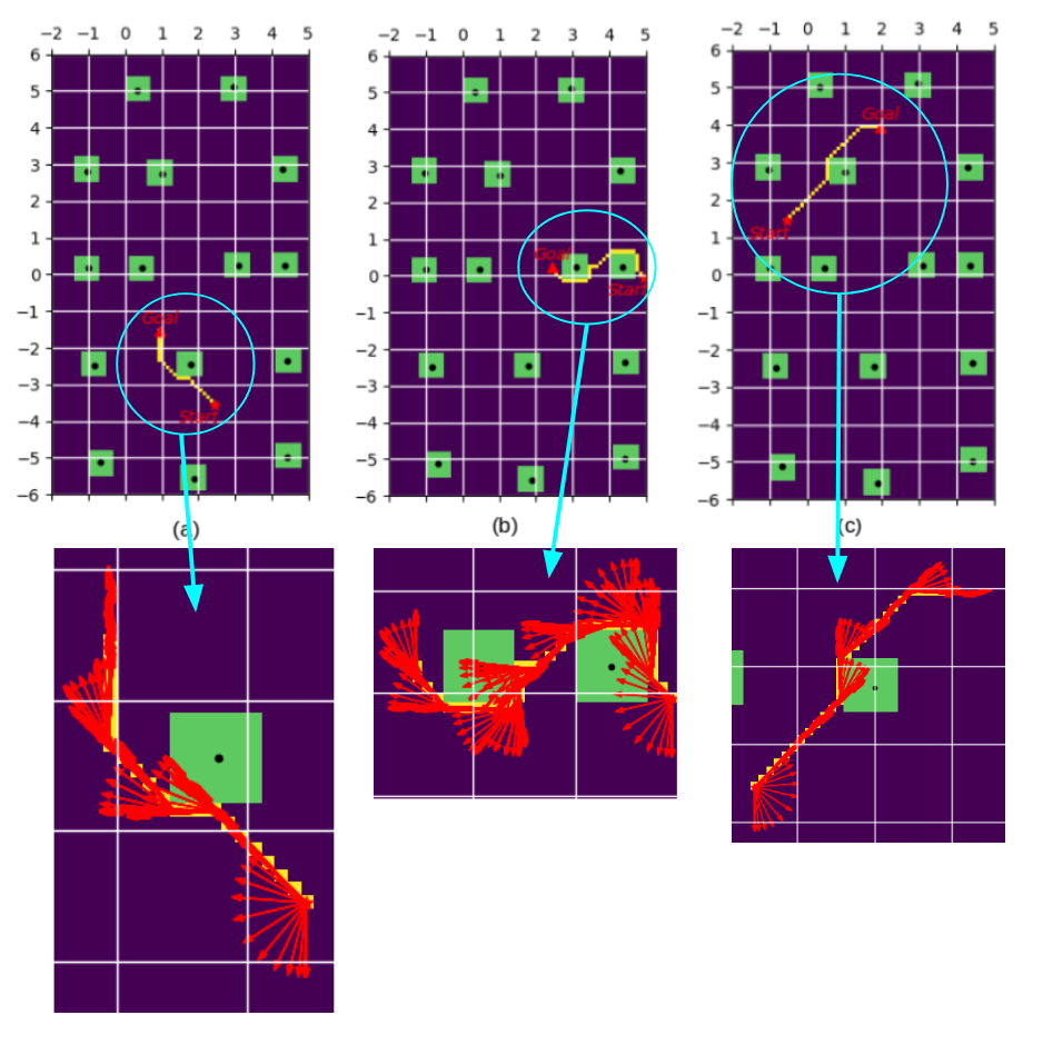
Now let’s work with a slightly more realistic grid, change path cell size to \(0.1m \times 0.1 m\), as shown on figure 5,the green boxes are the obstacles(size in \(1m \times 1 m\)), the yellow blocks are the path planned (size in \(0.1m \times 0.1 m\)) while avoiding obstacles.

Figure 4: Plan path base on online A star algorithm (a):S =[2.45,-3.55],G = [0.95,-1.55], (b): s=[4.95,- 0.05], G =[2.45,0.25], (c):S = [-0.55, 1.45],G = [1.95, 3.95]

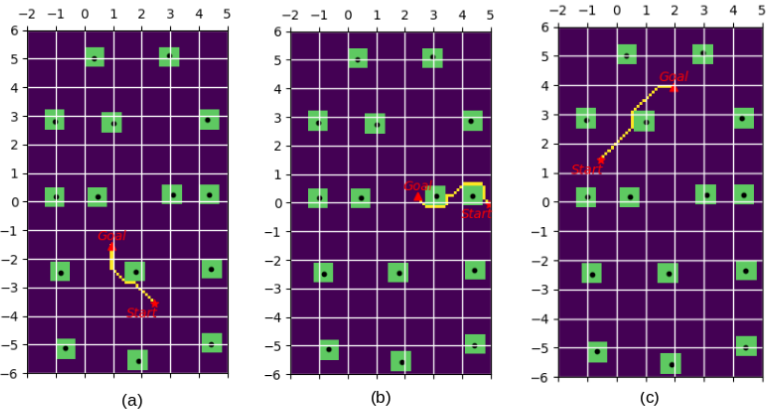
Figure 5 shows on the robot path planing from the start point to the end point, robot need to move along the node. Given the robot current 2-D position and heading \([x,y,\theta]\),(\(\theta\) is in range [0,2pi]),and the Target position \([x_T,y_T]\) it is needed to design a inverse kinematics which out put linear velocity and angular velocity \([v,\omega]\) The robot walk between two nodes are designed to do the rotation motion first, then do the linear motion. And the robot velocity at each node is 0.

The rotational motion:

\begin{equation} \phi = tan^{-1} (x_T , y_T) - \theta \end{equation}

If \(\pi>\phi >0\), robot need go clockwise;

If \(2\pi>\phi>\pi\), robot need go counterclockwise;

If \(-\pi<\phi<0\), robot need go clockwise;

If \(-\pi<\phi<0\), robot need go counterclockwise;

since \(\dot{\omega}_{max}\) = 0.288 , robot plan to increase the speed of rotation with max acceleration, with lowest acceleration, and keep the max speed for 0.1 second if necessary and then decrease sped of rotation with max acceleration.
Time for rotational motion: \begin{equation} T_a = 2\times\sqrt{\theta\over 0.288} \end{equation}

The rotational motion:round t with 1 decimal \begin{equation} T_a = round (T_a,1) \end{equation}

angular velocity: when \(0 < t < {T_a\over 2}\)

\begin{equation} \omega = 0.288 \times t \end{equation}

max angular velocity: \begin{equation} \omega_{max} = 0.288 \times{T_b\over 2} \end{equation}

angular velocity: \(T_a> t >{T_a\over 2}\)

\begin{equation} \omega = \omega_{max}- 0.288 \times t, \end{equation}

since \(\dot{v}_{max} = 5.579\),, robot plan to increase the linear speed with max acceleration, then keep the max speed for 0.1 second if necessary and then decrease linear speed to 0 with max acceleration.

Linear distance between two nodes: \begin{equation} S = \sqrt{(x_{T} - x)^2 + (y_{T} - y)^2)} \end{equation}

Total time of linear motion \begin{equation} T_b = 2\times\sqrt{S\over5.579} \end{equation}

Round T_b with 1 decimal place \begin{equation} T_b = round (T_b,1) \end{equation}

Linear velocity: when $ 0 < t < {T_b\over 2}$ \begin{equation} v = 5.579 \times t \end{equation}

max linear velocity: \begin{equation} v_{max} = 5.579 \times {T_b\over 2} \end{equation}

linear velocity:when \(T_b > t > {T_b\over 2}\) \begin{equation} v = v_{max}- 5.579 \times t \end{equation}

From the figure1, we can see robot is almost adhered with path planed by A star search, and it can optimize rotation direction by choosing its counter-clock wise or clock wise direction. However, sometimes robot’s heading is hard to match with exactly target node position. so setting a proper size of threshold is very important.

The code can be found on my github